GIS 4102 Module 10 - Creating Custom Tools

Learning about script tools this module was quite awesome. The use of parameters instead of hard-coded information as is used in stand-alone scripts provides so much flexibility and transferability of the script. Another advantage of script tools over stand-alone scripts is that message statements which are written to a progress dialog box and the Results window can be in a script tool. This allows the retrieval of results messages at a later time. Stand-alone script messages are printed to the interactive window and cannot be retrieved later. While the use of stand-alone scripts requires some knowledge of Python, the use of script tools does not require knowledge of Python. The script tool's dialog box is a convenient way for users to enter parameters with validation and error-checking included. The script tool window for this assignment is shown here:

Script Tool Window Showing Parameters Ready for Input

Even the creation of a script tool is relatively easy. After verifying that the stand-alone script forming the basis of the script tool works properly, a new script tool is added to a toolbox in ArcMap's Catalog. The new script tool is given a name, label, description, script file, and so on before parameters are added. After properties for each parameter are set, the original stand-alone script is edited to replace hard-coded filepaths or file names with the applicable parameters from the script tool. Print messages in the stand-alone script are replaced with message statements. This image shows the messages after running the tool for this assignment:

Resulting Messages from a Script Tool Which Clips
Several Layers to a Single Feature

Once the performance of the script tool has been confirmed, the script and toolbox containing the script tool can be zipped together into a folder. Voilà! It's ready to share with anyone else. Just for fun, I emailed the zipped file to myself and used it with some other data. Here's an image of Orange County, Florida, with roads and some other features clipped to the county line...another demonstration of the incredible functionality and adaptability of Python scripting:

Orange County, Florida, with Features Clipped Using Script Tool

GIS 4102 Module 9 Assignment: Debugging & Error Handling

Figure 1
First Script - List of Airports

Debugging and handling errors were emphasized in this week's module. Having experienced quite a bit of debugging my own scripts in this course, especially with syntax and using the technique of commenting out sections of code, this exercise and assignment were extensions of that but also included try-except statements. The first script, with results shown here, contained two relatively easy syntax errors which allowed the script to run after correction. A list of airports was printed as a result (Figure 1).

Finding the eight errors in the second script took longer. The errors in the second script included misspellings, incorrect punctuation, and arguments along with incorrect mxd and path names. Once corrected, the script printed out a list of layers in the data frame as shown in Figure 2.

Figure 2
Second Script - Layers in Data Frame

Although in retrospect it was relatively easy, the third script took the longest. This was due primarily to determining where to place the try-except statement which, once placed correctly, allowed the script to run through to completion with an error message being printed for Part A and select data frame properties being printed for Part B. These results are shown in Figure 3.

Figure 3
Third Script - Error Message and Specified Data Frame Properties 

The step-through mode of the debugger was quite helpful for this assignment. All the techniques for error and exception handling will be very useful in future assignments during the course and employment.

GIS4102 - GIS PROGRAMMING: Participation Assignment #2 ~ GIS for Monitoring Animal Diseases

GIS has been shown to be of benefit in the field of veterinary science. In her 2001 paper, "Geographical Information System (GIS) as a Tool in Surveillance and Monitoring of Animal Diseases", published in Acta Veterinaria Scandinavica, Madelaine Norstrøm overviewed the possibilities and potential uses of GIS with respect to animal diseases.

Along with a general description of GIS, Norstrøm noted that tables of information could be joined with geographical data utilizing a common identifier (ID). She mentioned that numbers are preferable for IDs to reduce the chance of misspellings with character variables. The easily understood format of a map can be used to report disease information (incidence, prevalence, mortality, and morbidity) at the farm, region or national level. Density maps can be used in movie format to show the spread of disease. Real time outbreak notification is possible as is updated information for farm personnel and reports for authorities and the media. This use would be especially beneficial during an emergency situation.

Western Fjord Cattle
Photo Credit:  Anna Rehnberg
http://sciencenordic.com/endangered-norwegian-livestock-hanging

Using GIS, the locations of the case farm and at-risk farms can be identified in the event of an infectious disease outbreak. Buffer zones can be created around these as well as other risk areas such as markets, roads, and slaughter houses. With this information, veterinary personnel can develop a plan of action. Norstrøm stressed the importance of performing a cluster analysis related to time and space to minimize misinterpretation of visual point patterns on maps. The integration of simulation models within a GIS utilizes risk factors for the spread of disease.

Norstrøm continued with an explanation of what data is available and where to obtain it. She mentioned that the goal is to have maps continuously displaying each disease's status. Norstrøm concluded with two specific examples of GIS use for specific swine and cattle diseases.

GIS 4102 – GIS Programming Module 8 – Working with Rasters

The purpose of this week's lab assignment was to produce a composite raster from 5 intermediate rasters which were created using various aspects of  the spatial analyst extension. After writing code to determine whether the spatial analyst extension was available, it was checked out, and the fun began. Three land cover classifications were assigned identical values; reclassification of the land cover raster was based on those new values. From the elevation raster four intermediate rasters were created based on slope and aspect values (slope between 5-20° and aspect between 150-270°). Finally, the five temporary rasters were combined into one raster which was saved, and the spatial analyst extension was checked in.

Final Raster Depicting Landcover Classification 1,
Slope 5-20°, and Aspect 150-270°

The main problem that I had with this particular script was that the outcome did not match the sample provided in the lab instructions. I had three colors in ArcMap instead of two. A big concern is that I would not have caught this error (since my script ran without trouble or messages) except that I was able to make this comparison and noticed the difference between my results and the lab instructions sample. The resolution of this issue turned out to be rather simple.

Because I remembered being confused by the inclusion of “NODATA” as a parameter in the reclassify portion of the lab exercise on p. 17 which is what I modeled my script on, I revisited that information in the text and learned that the 4th parameter is optional. I removed “NODATA” from my script, ran it again, and got the desired results, shown here.

With the completion of each lab, I am more impressed by what can be done in ArcMap with Python. I'm looking forward to the next lab!

GIS 4048 Urban Planning: GIS for Local Government

The study of local government continued with this lab which was composed of two scenarios.

Scenario 1 involved students as GIS Technicians employed by the Marion County Property Appraiser's office. The county property appraiser's website and online map were utilized to provide information to a local developer who was interested in the impacts a Fly-In Community would have on property owners adjacent to a specific parcel of land in the county. His request for a preliminary zoning report of the site and adjacent areas was met with a PDF map book and a PDF of contact information for the owners of parcels within 1/4 mile of the subject parcel. The map book was created with data driven pages and included an index map. Each page of the map book focused on one particular area that was overviewed in the index map. Although this project had to do with zoning, creating something reminiscent of DeLorme Atlas and Gazetteers was very gratifying. The fact that the pages are so easily editable is very exciting.

After verifying the certification date of the data, the appraiser's website was navigated to develop a familiarity with it. The Marion County Property Appraiser had very detailed information for the subject parcel. (Something that would have made my own dog quite jealous was discovering the assessed value of $6,500 on the property's doghouse.) This particular website allows the buffering of parcels and downloading of data in .csv format. This data was used to add parcel owners' names to the data already provided using Join in ArcMap. The colors for the different zoning classifications were selected to correspond to the actual colors used in the county property appraiser's zoning map. This would develop a familiarity and provide a reference to the client. Each parcel within a 1/4 mile of the subject parcel was assigned a Map Key identifier. These numbers were also used in the corresponding Parcel Report PDF. Compiling the map book involved using this data and a selection of parcels within 1/4 mile of the subject parcel coupled with the zoning information and streets for reference. The index map for the map book was created to identify which portion of the overall map was the focus of a particular page in the map book. Labeling in data-driven pages is something that I found to be more complicated than labeling  layers in a standard map. With more practice that, too, should become second nature.

After completion of the data-driven pages and addition of final touches to the map, the map was exported to a PDF file to be provided to the client. Also provided to the client was a corresponding report of the parcels (identified by Map Key) with parcel ID, owner's name and address, zoning code, and acreage. This report was in PDF form. Generating a report from the attributes will be a handy skill to have. One page of the multi-page map book is included here:

Preliminary Zoning Report - Parcel No. 14580-000-00 and Adjacent Areas
Sheet B4, Page 6 of 12 in Map Book 

The second scenario of the lab exercise involved providing Gulf County Board of County Commissioners with a PDF list of vacant, county-owned parcels greater than 20 acres which they could consider for the construction of a future Extension office. Completion of this task required merging two parcels and then using editing tools to separate out a portion of the new parcel using a legal description. The new parcel's attribute information was then updated along with the new acreages for each of the two parcels. Selecting by Attributes yielded 75 parcels owned by Gulf County. A Definition Query utilizing Query Builder yielded 11 properties of more than 20 acres. Finally, a Vacant-Improved Code (VICD) Table was joined to the layer, and from this three vacant parcels were located. The results were organized in an attribute report which was exported as a PDF to be provided to the Board of County Commissioners.

Urban Planning - GIS for Local Government: Participation Assignment

This final participation assignment involved performing as a GIS technician with a Property Appraiser's office.  The first part involved learning a bit about the way a property appraiser's office manages property data with GIS. This was followed by learning how to display parcel data in a fashion that allows for quick interpretation and comparison of data.

My home county is Escambia County, Florida, which has a property appraiser’s web mapping site at http://www.escpa.org/CAMAGIS/ along with a mobile version available as well (http://www.escpa.org/mobile/map/mapmain.html). The county also has data downloads available at http://www.escpa.org/MapMain.aspx.

June 2014 Property Sales

A search of Escambia County real estate records can be done by specific dates at http://www.escpa.org/cama/SaleSearch.aspx. A recent search for the month of June 2014 revealed that the selling price for the highest-selling property in Escambia County, Florida, in June 2014 was a whopping $6,000 on 6/18/2014. All other properties that were transferred in June 2014 had sale prices of $100.  That covers many different types of transfers, including quitclaim deeds, probate, etc. In Oct 2007 the aforementioned property was transferred by quitclaim deed for $100.

For the property mentioned above, the assessed land value is $4,560. With improvements, the total assessed value is $6,888. Usually I see assessed values lower than recent sales values, but this particular assessment is higher than the most recent sale price.

Sales Records and Assessed Values for One Property

Additional information about this property makes note that the improvements on the land consist of a mobile home. Also, this property had a tax deed transfer in 1999 for delinquent taxes. That this was the highest selling property (at the time I accessed the information) for a whole month in Escambia County is interesting.  Some of the $100 “sales” (quitclaim transfers of property) were because of probate situations; others might have been transfers as the result of divorce settlements.

The second part of the participation assignment involved generating a map showing the assessed land values for a subdivision in Escambia County, Florida. IMHO, showing easements across properties is a good idea in that it indicates the extent of a factor which could negatively impact the worth of a property. Easements may give rights to access, construction, and maintenance of utility lines along with other purposes. Given two otherwise identical lots, the lot which has a utility easement across it should be valued less since the owner would not have full use of that area.

West Ridge Place - Land Assessment Values (2011)
Escambia County, Florida

Several lots in West Ridge Place subdivision should be considered for re-assessment:

• Lot # 090310165 is assessed more than $6,000 higher than all other lots in its vicinity.
• Lot # 090310290 should be re-assessed as well to be more in alignment. Like Lot # 090310105 across the street, this lot is impacted by three different easements. A lower assessed value may be justified.
• If Lot # 090310410 is not an easement of some kind, then it should be re-assessed for being significantly lower in assessed value even though it is quite a bit larger than other lots in the subdivision.

Because there is no road frontage on Mobile Highway or Chester Drive for Lot # 090310420, it appears to be one of the easements mentioned in the introductory material.

To someone who is interested in monitoring the home values of her own neighborhood, much of the experience of roaming around a property appraiser's web site was quite familiar already. I know how much the recent sales were, who owns the vacant house on the corner, who owns the house that's being used as a drive-up drug store (we're not talking Walgreens here), etc. Life in the 'hood. There's always something going on...

GIS 4102 – GIS Programming Module 7 – Working with Geometries

The assignment for this week's module involved creating a text file with data from a rivers shapefile. This turned out to be a greater challenge than creating a shapefile from a text file. Before committing my scripting results to the text file, I worked out the kinks with just a version printed to the interactive window. After it was printing the proper results, I went back and added the write command. The pseudocode for this assignment is shown below along with a portion of the resultant text file:

Start

Text File Created from a Shapefile

Import modules & classes

Set workspace

OverwriteOutput

Set output path

SearchCursor (OID, SHAPE, NAME)

Open text file

Processing statement

Row Loop

        Set vertex counter

        Point Loop (getPart)

        Increase counter

        Print row

        Write row to text file

Process complete statement

Close text file

Delete row

Delete cursor

End

This scripting turned out to be more challenging than I expected. Something that I found helpful was to comment out certain sections of code while I was making adjustments. That way not only did I preserve code that was working, but I also could alter other code to get the results I needed.

GIS4048 Location Decisions – Homing in on Alachua County

This module's lab exercise had students performing as consultants for a professional couple relocating to Gainesville in Alachua, Florida. Their goal is to find a home that is not only convenient to both workplaces (North Florida Regional Medical Center and University of Florida) but also is in a neighborhood of primarily owner occupants in their 40s. To accomplish this required demographic information from the US Census as well as school and medical facility datasets.

Analysis of Potential Home Locations by Different Criteria

With this information, the Euclidean Distance ("as the crow flies") tool first was used to generate distance zones around the hospital and then again around the university. Each of these raster layers was then reclassified to defined intervals to obtain ranked values. Identical color ramps were selected for easier comparison between data frames. The age and ownership layers were generated by adding fields to the applicable attribute tables and then using the field calculator to determine percentages. Again, the color ramps were selected so that the least ideal areas were shown in cool colors and the most ideal colors were shown with warm colors for easier comparison. These four data frames are shown on the first map with 3 census tracts meeting the ideal condition highlighted in each data frame.

The second map is composed of data frames created using the Weighted Overlay tool.  A model was utilized for this part with each factor given equal weight in the model. The usefulness of a model was demonstrated when the imaginary couple decided that they really didn't want to deal with Alachua County traffic after all and would prefer to find a home closer to work. The model was adjusted, giving higher weights for proximity to work and lower weights to the age and ownership criteria.  Changing values like this to accommodate a client's reconsiderations took very little time or effort.

Weighted Analyses of Potential Home Locations

A base map was included as an additional, separate map. After trying to pack all the above information into two maps, it became obvious that a larger format would have been a wise choice. Using weighted analysis is applicable not only to location selection for a residence, but also to determine feasibility studies including suitability of sites for farming, construction of a high-rise or ski slope, and so on.

GIS4048 Module 7: Homeland Security - MEDS Protect

Three Mile Buffer Zone around Boston Marathon Finish Line
with Nearest Hospitals and Finish Line Perimeter Security Checkpoints

Lessons learned from the 2013 Boston Marathon bombing have prompted increased security measures by the Department of Homeland Security. These measures include increased security at ingress and egress points as well as improved surveillance around the event site for monitoring purposes. The first map created for this exercise shows a 3-mile buffer zone around the Boston Marathon finish line, a 500-foot buffer around the finish line, the locations of the ten nearest, currently operational hospitals with emergency rooms, and their 500-foot radius protective buffer zones within which increased security measures prior to, during, and following the marathon can be planned. Fifteen security checkpoints on local and secondary roads leading to the finish line are shown at the outer limit of the 500-foot buffer zone around the finish line as shown on the smaller inset map. Identification verification and backpack checks could take place at those locations.

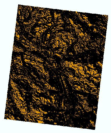
The second map focused on specific locations suggested for placement of surveillance equipment within the immediate vicinity of the finish line itself. LAS Dataset 3D View and the orthoimagery layer were used to determine where to place the 15 potential surveillance points. Prior to point selection, hillshade was generated for 2:30 pm on April 15, 2013. Shadows impact surveillance equipment's capabilities, and hillshade provided a baseline for the day of the marathon. A difficulty encountered during selection of surveillance locations was determining a set of locations that would provide complete coverage of the finish line vicinity as determined by using the Viewshed tool. Viewshed is an indicator of visibility from other vantage points, in this case, surveillance locations. Believing that cameras placed along roof lines or on the sides of buildings would provide that coverage, initial points were placed in that manner. However, to obtain fairly contiguous coverage, the points had to be adjusted not only vertically but also horizontally. Not knowing the heights of the buildings in the area was a disadvantage, but taking advantage of Google street view as well as researching commercial building heights in general provided some guidelines to estimate reasonable, attainable heights for surveillance cameras. Using 3D GIS techniques to determine locations of surveillance points is significantly more economical, effective, and efficient time-wise than physically selecting, inspecting, and adjusting potential surveillance points.

Suggested Locations for Surveillance Points near Boston Marathon Finish Line

The biggest roadblock that I encountered in trying to assemble a comprehensive security analysis for the marathon came with the inability to complete the line-of-sight portion of the lab. Even with meticulous attention paid to the line-by-line instructions and completing the work in one session (having been forewarned), I could not get a line of sight to show up between any pair of selected points (any surveillance point and the finish line). Redoing the map from the very beginning several times, including completely re-downloading the data again did not improve the situation. This resulted in an incomplete map as a profile graph could not be made for a nonexistent line of sight. Having a profile graph would have enabled a surveillance team to further evaluate potential surveillance points. For instance, the horizontal location of the obstruction can be determined by the aerial view, but how the obstruction possibly could be lessened by the vertical adjustment of the surveillance camera can only be determined by a side view shown with a profile graph.

A 3D version of the map was created in ArcScene using the finish line raster as a surface layer. The orthoimagery layer was draped over it as well. Because I did not have any lines of sight to put in the ArcScene portion of the lab, I added the finishline and suggested surveillance points, hoping that the surveillance points would be placed at their offset heights. That did not happen. Again, the actual line of sights are an essential part of a security analysis like this.

Even though I was unable to complete the lab as intended, the experience was extremely worthwhile. The numerous repetitions of certain steps have helped reinforce key aspects of the lab.

GIS 4102 GIS Programming Module 6: Explore/Manipulate Spatial Data

First Portion of Results

The assignment for this module started with a script template which was expanded using the skills learned in the exercise portion of the module. Provided shapefiles were stripped of their .shp extensions and added to a new geodatabase by a scripted for loop. A search cursor was used to retrieve only those cities identified as county seats in the "FEATURE" field of the cities layer . Another for loop was used to populate a newly created dictionary with the names and populations of those county seats. The results of the script are shown in this series of screenshots.

Middle Portion of Results

A troublesome spot I encountered was being unable to delete my geodatabase after having run the script multiple times. That “Failed to delete…” error message became a bit annoying. Initially I started deleting feature classes individually, and then discovered that I could not delete the “cities” layer because of a schema lock. After reviewing schema locks in the text, it became clear that del row and del cursor needed to be included.

The next part of this problem came up: how to run the script with the changes if the geodatabase could not be deleted until the lock was lifted which could not be done without creating a geodatabase. Vicious cycle, I say. A temporary geodatabase was created, del row and del cursor were added to the script, the original geodatabase was unlocked, and deleted. The temporary geodatabase was also deleted, and the script was revised back to the name of the original geodatabase. All of this would have been unnecessary had I remembered to close ArcMap before running Python script. C'est la vie! I'll remember that now!

Final Portion of Results